The Sixth Assessment Report of the Intergovernmental Panel on Climate Change (IPCC AR6) has been released, much to the excitement of and fanfare from the mainstream media.  It was expected that gloom and despair would permeate the document – unless, of course, we adopt a draconian carbon-dioxide-reduction strategy – and the IPCC did not fail to deliver.

So, where do these extreme climate scenarios originate?  One could assume that they could be “made up”; after all, climate change science has long been plagued by Maier’s Law – if the data do not conform to the theory, the data must be discarded.  But scientists need to show something for all the money they are spending on climate change; thus, creating climate models allows climate modelers to earn their keep.

Unlike model airplanes or trains, a climate model is not a physical manifestation, but a mathematical representation of the climate system.  One assumes that we take all the equations that describe everything related to climate, convert them to computer code, press the “RUN” button on the computer, and sit back and discover that the Earth will become a fireball in a very short time – unless we take extreme measures to stop increasing concentrations of atmospheric carbon dioxide.

Well, that is not quite how it works.  In 2007, the Workshop on Theoretical Alternatives to Climate Modelling noted that “contrary to a widely held misconception, computer modeling of climate is, to a large degree, based on empirical rules of thumb and uncontrolled approximations in many of its key physical aspects” (emphasis original).  A decade later, climate modelers finally admitted in The Art and Science of Climate Model Tuning that

“With the increasing diversity in the applications of climate models, the number of potential targets for tuning increases.  There are a variety of goals for specific problems, and different models may be optimized to perform better on a particular metric, related to specific goals, expertise or cultural identity of a given modeling center.” (Emphasis added)

Models are optimized according to specific agendas?  Is this science as we knew it, or is it post-normal science where “expertise” guides the outcome?

The only true way to evaluate a climate model is to compare it with observed data.  One might assume that we take thermometer data and compare it to the modeled time series.  But, as a famous climate alarmist[1] once said, “The data are dirty!”  And indeed, they are!  Our thermometers are located predominantly over land, in mid-latitudes, at lower altitudes, in more affluent societies, and along coastal regions – in short, where developed people live.  Few measurements exist over oceans, high latitudes, deserts, and the tropical rainforests.  Moreover, many of their records are incomplete or biased due to station moves and discontinuities, changes in instrumentation, and bad siting practices.  Moreover, they measure only the air temperature at about 5.5 feet – a convenient height for a six-foot weather observer to access the station.

As a result of the inadequacies of station observations, climatologists often use satellite data.  Although satellite estimates of air temperature exist only since 1979, they do provide a near complete spatial coverage and integrate the atmospheric temperature over the lower troposphere, not just at 5.5 feet.  Thus, satellite estimates of atmospheric air temperature are preferable to and relatively accurate when compared to disparate thermometer networks.

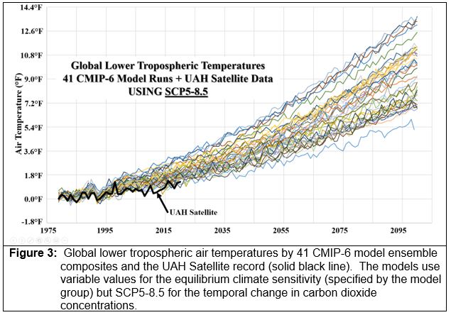
When model simulations of the current climate (1979 to 2020) are compared with the satellite record, climate models tend to run “hot”; that is, models usually overestimate the increase in air temperature over time relative to that observed by the satellites.  Indeed, Dr. John Christy has testified to both houses of the United States Congress regarding to the extent to which climate models overestimate the rate of air temperature increase over time. Why is that?  We can discuss the application of convective parameterization by the models, the spatial averaging process that affects computer simulations, uncertainties associated with parameterizing ice sheet dynamics – but these are highly technical, scientific explanations. 

At a very basic level, however, there is a very simple explanation as to why models run hot – and it is given by this very basic equation:

where the change in air temperature over time, in the models is explained by two simple terms.  I will show that both terms are overestimated, which contributes to the overestimation of the climate sensitivity (the term on the left of the equal sign).

The first term,

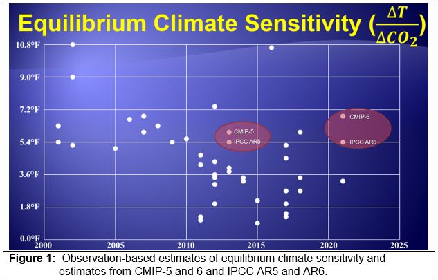
, describes the model response in air temperature to a change in carbon dioxide concentrations.  This term can be described as the transient climate response (TCR) or the equilibrium climate sensitivity (ECS), depending on whether a transient value or steady-state solution is considered.  Charney in 1979 and the First Assessment Report of the IPCC both assumed that ECS fell between 2.7°F and 8.1°F for a doubling of carbon dioxide.  Early estimates in the 2000s suggested average values between 9°F and 11°F, although most other estimates ranged between 4.5°F and 7°F for a doubling of carbon dioxide.  Since then, however, observational estimates of ECS have dropped dramatically to values that may be less than 2°F, although models and the IPCC Sixth Assessment Report still suggest the ECS is about 5.5°F (Figure 1).

Thus, the first term in the equation – climate sensitivity – is overestimated by both the models and the IPCC, relative to independent estimates obtained from observations. The second term,

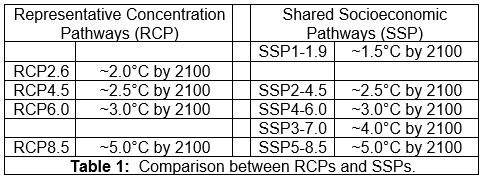
, describes how the model simulates the increase in carbon dioxide over time.  In previous years, four scenarios were posited:  RCP2.6, RCP4.5, RCP6.0, and RCP8.5.  RCP is “Representative Concentration Pathway” and the number after is the anthropogenic forcing (in Wm^-2) that occurs by 2100.  More recently, five basic scenarios have been suggested:  SSP1-1.9, SSP2-4.5, SSP4-6.0, SSP3-7.0, and SSP5-8.5.  SSP is “Shared Socioeconomic Pathway”, the first number is the socioeconomic challenge (1-Sustainability, 2-Middle-of-the-road, 3-Regional Rivalry, 4-Inequality, and 5-Fossil Fueled Development), and, as before, the second number is the anthropogenic forcing by 2100.  The following table (Table 1) compares the two methodologies.

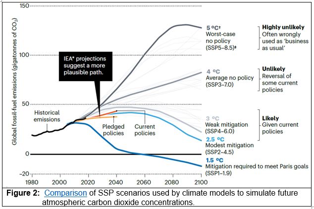
The IPCC AR6 uses these SSPs to model possible energy usage and, consequently, the emission of greenhouse gases.  Many scientists interpret a “business-as-usual” scenario as SSP5-8.5 (or RCP8.5) with all other scenarios resulting from some degree of restriction of greenhouse gas emissions.  This is not an appropriate interpretation as the SSP3-7.0 and SSP5-8.5 scenarios are considered “unlikely” (Figure 2).

Unfortunately, most model evaluations of future climate scenarios utilize SSP5-8.5 (or previously, RCP8.5) to simulate the effect of changes in atmospheric carbon dioxide.  Note that Hausfather and Peters (Figure 2) identify this scenario as being “highly unlikely.”  Nevertheless, this extreme scenario generates extreme changes in most climate variables, which is exactly what climate alarmists want to see. Thus, the model representation of the change in air temperature over time—

—is overstated (i.e., “runs hot”) because most model simulations use (1) an ECS that is too high—

—relative to observations and (2) a scenario for changing atmospheric carbon dioxide concentrations—

—that is admittedly “highly unlikely”.  It makes for a very dramatic presentation with considerable warming occurring by 2100 (Figure 3).

---

[1] Professor Thomas Wigley, Personal Communication